Appendix
Obtaining information from QC packages
In the following part, we aim to introduce how to obtain useful calculation results from other QC packages. We use 1,4-distyrylbenzene molecule (DSB, Configuration of DSB ) and Gaussian 09 package to illustrate the points.
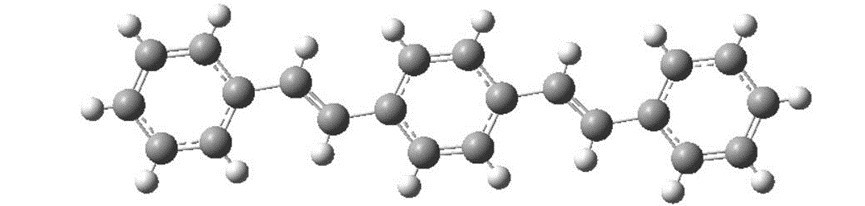
Configuration of DSB
Gaussian 09 is used to handle optimization and frequency calculations on ground state (\(S_0\)) and lowest singlet excited state (\(S_1\)), transition dipole moment and transition electric field between \(S_0\) and \(S_1\) states.
Optimization calculation on ground state (\(S_0\))
After constructing the initial geometry, we have to find the optimized
\(S_0\) geometry. The route section is set as
#p opt b3lyp/6-31g*, which indicates an optimization calculation at
B3LYP/6-31G* level.
When the calculation is completed, find the last line with “SCF Done” in
the output *.log file in order to find single point energy at the
optimized \(S_0\) geometry. In this example, the last line with “SCF
Done” is the following:
SCF Done: E(RB3LYP) = -849.172438992 A.U.
Complete results can be found in directory
examples/DSB/opt_and_frequency.
Frequency calculation at the optimized \(S_0\) geometry
After finding the optimized \(S_0\) geometry, we need to verify the
optimization result and calculate its force constant matrix via
frequency calculation. The route section is set as
#p freq b3lyp/6-31g*, which runs a frequency calculation at
B3LYP/6-31G* level. You have to define the location of *.chk file
in Link 0 Commands as well.
Use Gaussian built-in command formchk to generate a *.fchk file
based on output
*.chk. The *.fchk file contains readable force constant matrix
information that is needed in evc calculation.
Complete results can be found in directory
examples/DSB/opt_and_frequency.
In this example, the route section is set as
#p opt freq b3lyp/6-31g*, which means we run optimization and
frequency calculations at the same time. But we recommend separating
them into two types of calculation in order to avoid any possible
mistakes.
Transition dipole moment (absorption) at the optimized \(S_0\) geometry
After finding the optimized \(S_0\) geometry, we can calculate
transition dipole moment (absorption) and vertical excitation energy at
this geometry. The route section is set as #p td b3lyp/6-31g*, which
runs a calculation at B3LYP/6-31G* level using TDDFT method.
When the calculation is completed, find the relative information about
“Excited State 1” in the output *.log file in order to find vertical
excitation energy and transition dipole moment (absorption) at the
optimized \(S_0\) geometry. In this example, the information is
listed below:
Ground to excited state transition electric dipole moments (Au):
      state          X           Y           Z       Dip. S.     Osc.
        1        -4.6693     -0.0118      0.0112     21.8029    1.7826


Excited State   1:      Singlet-A   3.3372 eV   371.52 nm   f=1.7826  <S**2>=0.000
     75 -> 76         0.70728
This state for optimization and/or second-order correction.
Total Energy, E(TD-HF/TD-KS) =  -848.655200149
Hence, vertical excitation energy at the optimized \(S_0\) geometry
is 3.3372 eV, and transition dipole moment (absorption) can be obtained
using Dip. S.:
Optimization calculation on lowest singlet excited state (\(S_1\))
With the optimized \(S_0\) geometry, we can start optimizing
\(S_1\) geometry using the optimized \(S_0\) geometry as the
initial structure. The route section is set as
#p td opt b3lyp/6-31g*, which indicates an optimization calculation
at B3LYP/6-31G* level using TDDFT method.
When the calculation is completed, find the last line with “SCF Done” in
the output *.log file in order to find single point energy at the
optimized \(S_0\) geometry. In this example, the last line with “SCF
Done” is the following:
SCF Done: E(RB3LYP) = -849.165742659 A.U.
Complete results can be found in directory
examples/DSB/opt_and_frequency.
Frequency calculation at the optimized \(S_1\) geometry
After finding the optimized \(S_1\) geometry, we need to verify the
optimization result and calculate its force constant matrix via
frequency calculation. The route section is set as
#p td freq b3lyp/6-31g*, which runs a frequency calculation at
B3LYP/6-31G* level using TDDFT method. You have to define the location
of *.chk file in Link 0 Commands as well.
Use Gaussian built-in command formchk to generate a *.fchk file
based on output *.chk. The *.fchk file contains readable force
constant matrix information that is needed in evc calculation.
Complete results can be found in directory
examples/DSB/opt_and_frequency.
Transition dipole moment (emission) at the optimized \(S_1\) geometry
Transition dipole moment (emission) and vertical excitation energy at
the optimized \(S_1\) geometry are also given when the calculation
in section 7.4 is completed. Find the relative information about
“Excited State 1” in the output *.log file in order to find vertical
excitation energy and transition dipole moment (emission) at the
optimized \(S_1\) geometry. In this example, the information is
listed below:
Ground to excited state transition electric dipole moments (Au):
      state          X           Y           Z       Dip. S.     Osc.
        1        -5.3165     -0.0242      0.0000     28.2653    1.9597


Excited State   1:      Singlet-?Sym    2.8300 eV   438.11 nm   f=1.9597  <S**2>=0.000
     75 -> 76         0.71066
This state for optimization and/or second-order correction.
Total Energy, E(TD-HF/TD-KS) =  -849.061743778
Hence, vertical excitation energy at the optimized \(S_1\) geometry
is 2.8300 eV, and transition dipole moment (emission) can be obtained
using Dip. S.:
and transition dipole moment (absorption) can be obtained using
Dip. S.:
Complete results can be found in directory
examples/DSB/opt_and_frequency.
Adiabatic energy difference between \(S_0\) and \(S_1\) states
The adiabatic energy difference between \(S_0\) and \(S_1\) states can be calculated using single point energy results from sections 7.1 and 7.4.
In this example, the adiabatic energy difference is:
Transition electric field and NACME at the optimized \(S_1\) geometry
After finding the optimized \(S_1\) geometry, we can calculate transition electric field at this geometry. Then it’s possible to run a evc calculation with NACME option toggled on.
The route section is set as the following line:
#p td b3lyp/6-31g(d) prop=(fitcharge,field) iop(6/22=-4, 6/29=1, 6/30=0, 6/17=2)
When the calculation is completed, copy two output *.log files into
a new directory. One is transition electric field *.log file, which
is obtained in this section. The other is frequency calculation at the
optimized \(S_0\) geometry *.log file, which is obtained in
section 7.2. Then use get-nacme to start calculating NACME.
Complete results can be found in directory examples/DSB/nacme.